Strategy for improved the characterisation of human metabolic phenotyping using COmbined Multiblock Principal components Analysis with Statistical Spectroscopy (COMPASS)

We have recently published a strategy for improving human metabolic phenotyping using Combined Multiblock Principal components Analysis with Statistical Spectroscopy (COMPASS). The COMPASS approach is developed within R environment. The open access manuscript can be found here.

In this blog, we describe how to get started.

Characterising and understanding how human phenotypes relate to population statistics requires the ability to ascertain the occurrence of certain traits in individuals from different populations. For NMR and MS spectroscopic based datasets, this means the ability to estimate the presence of a specific feature, aka a signal, across the whole dataset (population) and aggregate the results by sub-population. In doing so, we can estimate the occurrence that varying between populations. For example, if interested in type-2 diabetes in a population we could observe how the anomeric doublet at 5.23 ppm vary across sub-populations. As NMR measurement is quantitative, the ideal solution for estimating the presence of a specific metabolite is to quantify the concentrations of that metabolite. However, this is not always as trivial as it sounds, partially because of peak overlap. To overcome this, COMPASS estimates the presence or absence of a signal, aka a trait, by computing the cross-correlation of a feature and comparing it against a “reference”. The “reference feature” (pattern /signal) is a feature of interest and this can be selected from the multivariate data analysis modelling pipeline. We will show you how to do this.

To run the COMPASS, it requires two R packages, MetaboMate for multivariate analysis and hastaLaVista for interactive visualization. Instruction for installing both packages, please refer to the README files provided with both packages.

Data modeling

In the github.com/cheminfo/COMPASS repository, a demo dataset and file multiblocking.R is provided to illustrate the functionality of COMPASS. This script will run multiple principal component analysis (PCA) models, each with a block of 0.5 ppm. If desired, the user can modify the block size in line 24 of this demo file.

# define the blocks (here blocks of 0.5 ppm are preferred)
rangeList <- list(c(0.5, 1.000), 
                  c(1.0005, 1.5), 
                  c(1.5005, 2), 
                  c(2.0005, 2.5), 
                  c(2.5005, 3), 
                  c(3.0005, 3.5), 
                  c(3.5005, 4.0), 
                  c(6.5005, 7),
                  c(7.0005, 7.5),
                  c(7.5005, 8),
                  c(8.0005, 8.5),
                  c(8.5005, 9),
                  c(9.0005, 9.49))

For very large datasets (typically file size of > 0.5 GB), loading of the dataset into the interactive visualisation web browser may become impractical. Thus, , hastaLaVista can be configured to retrieve spectra only when necessary. To do this, uncomment lines 45-53 and define a path to store the JSON. This will convert spectral data into an individual JSON file, thus enabling fast and efficient interaction of the browser. However, to do this, you must locate the folder where hastaLaVista is stored in your installation. This is achieved using the .libPathts() command and then creating the folder visu/data/json. Line 46 of the demo file must point to this json folder. Running the script will point your default browser on the URL.

http://127.0.0.1:5474/?viewURL=http://127.0.0.1:5474/view/modelExplorer_1_1.view.json&dataURL=http://127.0.0.1:5474/data/multiblocking.data.json

and you should see the following page where you can explore the scores and loadings for each of the block PCA models, the results for the whole PCA, together with the super scores and superloadings that are reconstructed based on combining all the scores and loadings for all the blocks. Using Alt-click it is possible to select scores and then select spectra that the user wants to display.

This visualisation tool allows the user to explore the dataset with a high level of granularity to define the features of interest.

Feature identification and selection

A useful feature of the vista is to allow the user to select spectra from the scores plot and the use these data to compute a Statistical TOtal Correlation SpectroscopY (STOCSY) model which finds all the correlated peaks relating to the feature of interest. The driver peak used to compute STOCSY is simply set by Alt-click on the selected spectra, on the corresponding variable (see video below). A STOCSY trace will appear in the middle gray area that allows the user to identify features that belong to the same molecule.

Computing cross-correlation

In the github.com/cheminfo/COMPASS repository, a demo MBCC-metaboliteX.Rmd file is provided to work with the provided demo dataset.

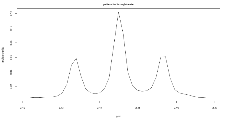
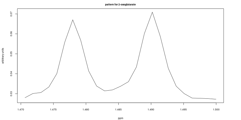
The following code chunk from the demo file (line 49 – 57) allows the user to select the feature that will be used as a reference. In this example we selected two features, a triplet between 2.42 ppm to 2.47 ppm; and a doublet between 1.47 ppm to 1.50 ppm. Both features are well resolved in the first sample (ID = 1). i.e. they are used as reference features to compute cross-correlation.

patternID <- 1
identifier = ID
L = length(ID)

# several ranges may be defined and combined to create a pattern
# define here the range that should be used
F <- which(x_axis > 2.42 & x_axis < 2.47)
F2 <- which(x_axis > 1.47 & x_axis < 1.5)
rangeList <- list(F, F2)

The reference features are shown here:

And finally we can compute and display the cross-correlation using the following code chunk (line 89 – 125 in the demo file).

# define here what information should be used as a category or a group
colorCode <- metadata$Class

ccList = list()

for (i in seq_along(rangeList)) {
  F <- rangeList[[i]]
  subX <- X[, F]
  
  pattern <- as.numeric(subX[which(identifier == patternID),])
  
  pattern[pattern == 0] <- 1e-04
  dil.F <- 1/apply(subX, 1, function(x) median(x/pattern))
  subX.scaled <- subX * dil.F
  
  res <- apply(subX.scaled, 1, function(x) {
    ccf(pattern, x, lag.max = 10, plot = FALSE, type = c("correlation"))
  })
  
  r <- unlist(lapply(res, function(x) max(x$acf)))
  par(mar=c(4,4,2,4))
  plot(r,
       main = paste0(metabolite, ": cc colored by country (pattern: ", patternID, ")"),
       xlab = "sample index",
       ylab = "cross-correlation",
       cex.main = 2,
       cex.lab = 2,
       cex.axis = 2,
       cex = 2,
       col = colorCode)
  ccList[[i]] <- unname(r)
}

The results of the cross-correlation for the triplet at 2.445 and doublet at 1.484 are plotted in figures below and color coded according to class:

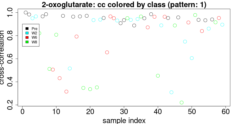
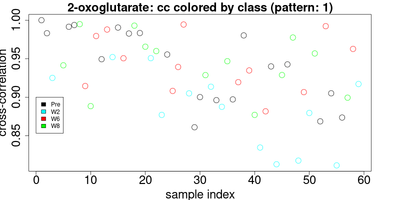
Definition of the cross-correlation limits to select features

These figures enable the user to define the level of cross-correlation. Although cross-correlation is insensitive to chemical shifts, it is however sensitive to distortions of the pattern due to overlap. Therefore it is necessary to visually inspect the results. Since this inspection is mandatory and cumbersome, we have made efforts to provide the best interface to quickly visually check the results.

The 2 thresholds are defined on line 137 and 139 of the script:

# define here the threshold for selection
selectThreshold <- 0.8
# define a threshold for coloring. The samples with cross-correlation below this level (lower confidence) will be displayed with red color later.
colorThreshold <- 0.9

In the upper figure (triplet pattern) a cross-correlation threshold may be easily defined at > 0.8. In the second case (doublet), the cross-correlation threshold is somewhat ambiguous. It is recommended that we choose to combine several (as many as possible) patterns and compute the combined cross-correlation, since the more complete the pattern, the better-defined the distribution of cross correlation will be. However, the noise may be another factor that impacts the cross-correlation level. For high-intensity signals, the cross-correlation values are usually higher than those signals close to the noise.

Visual inspection of the results

** The visual inspection is a mandatory step in the proposed method that is not intended to be fully automated!**

To visualise the results, the user has two options, printing the results using the script (lines 145 to 181), or use hastaLaVista (lines 213 to 240). In the first approach, the cross correlation (CC) thresholds are defined in the demo script (line 137 and 139). The feature region will thus be highlighted with green dots for spectra with CC above the hightest threshold, orange where the CC is between the two limits and red below. This traffic light system allows the user to quickly check the results.

Inspection using static images

Examples of figures generated using the first approach are shown below for the triplet at 2.445 ppm.

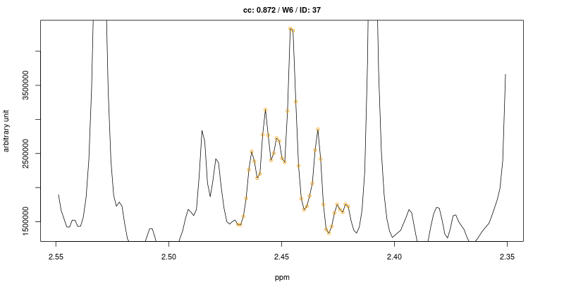
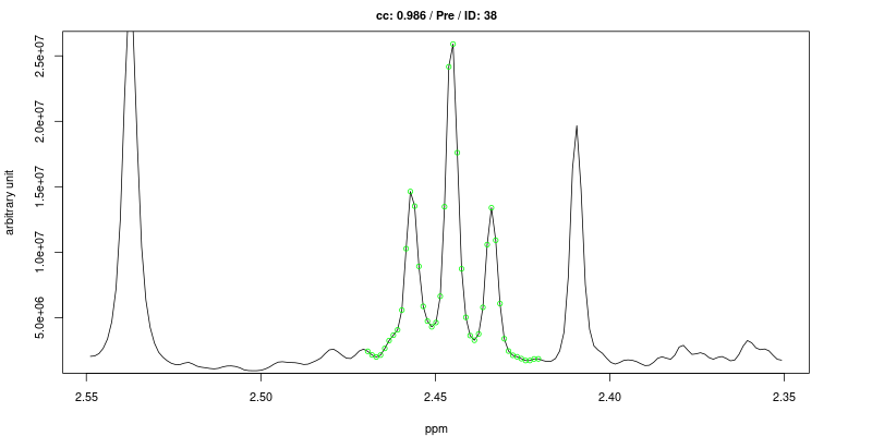
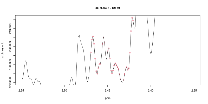
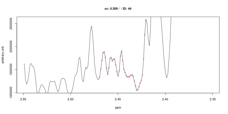
As expected the cross-correlation is not sensitive to the shift (second trace) of the triplet but is sensitive to overlap (top trace). Last two traces show CC for cases where no signal is present.

Interactive inspection of the results

A drawback of this approach is that the script has to be run each time a different threshold is defined. Since the threshold has to be accurately set and results thoroughly checked afterwards in order to produce faithful results, we provide a more interactive tool that enable interactive exploration of the results.

The second option makes use of the hastaLaVista package to make the visualization interactive, as shown here:

This visualisation tools enable the user to easily observe the resulting selection of CC threshold by moving a slider, and then to rapidly review the selected features over the whole dataset by simply choosing from the table.

For this example, by choosing a threshold at 0.8 the triplet feature is found in all 19 samples pre operation, while only found in 71% (10 out of 14) of the samples after 2 weeks, 46% (6 out of 13) after 6 weeks and 62% (8 out of 13) after 8 weeks.